paraxial parameters

For both refractive and reflective systems, algebric distances and dimensions transverse to the optical axis are positive from bottom to top. Algebric distances and dimensions along the optical axis are positive from left to right. In the following paragraphs and tutorial pages, considered systems are made of refractive and/or reflective surfaces also called optical surfaces or facets. When a spherical surface is considered, radius of curvature is measured from the curved surface vertex to its center.

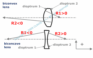As an example, for a biconvex lens, the radius of curvature R₁ of the first surface ( or facet ) is positive and the radius of curvature R₂ of its second surface is negative.

As another example, for a biconcave lens, the radius of curvature R₁ of the first facet is negative and the radius of curvature R₂ of the second facet is positive.

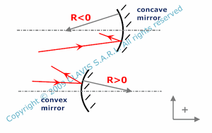A concave mirror has a negative radius of curvature R.

A convex mirror has a positive radius of curvature R.

A short definition of the transverse magnification (or more simply the magnification) detailed further is necessary at this stage. Let consider a punctual off-axis object A, its conjugated through the optical system A_i, d and d_i the respective algebric distances from the axis to A and A_i. The magnification is the ratio d_i/d.

Paraxial parameters are defined both in the object space (before the optical system) and in the image space (after the optical system). They are related to what are called the principal planes and the focal planes.

The principal planes are two planes perpendicular to the optical axis O_a. The secondary principal plane H_i (which is in the image space) is the paraxial image by the optical system and with a magnification of +1 of the primary principal plane H (which is in the object space). This means that an incident light ray intersecting H at the height h produces an emergent ray intersecting H_i at the same height h.
The object nodal point N and the image nodal point N_i are the intersection of the optical axis respectively with H and Hi.

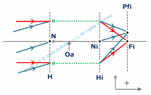The focal planes are also perpendicular to the optical axis. The conjugated of the front focal plane P_f (which is in the object space) is a plane perpendicular to the optical axis and located at infinity (left scheme on the left side). The conjugated of a plane located at infinity and perpendicular to the optical axis is the back focal plane P_fi (which therefore is in the image space - right scheme on the left side). The front focal point F is the intersection of the front focal plane P_f with the optical axis O_a.

Accordingly, its paraxial image is at infinity and on the optical axis O_a, which means that incident rays coming from F produce emerging rays all parallel to the optical axis O_a.

The back focal point F_i is the intersection of the back focal plane P_fi with the optical axis. Accordingly, it is the paraxial image of the on-axis point at infinity , which means that incident rays parallel to the optical axis are all converging to F_i after propagation through the optical system.

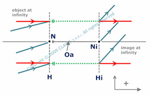There are particular optical systems which focal planes are at infinity. They are called afocal systems. In this case, the image of an object at infinity is also at infinity. Therefore, after propagating through the optical system, an incident collimated beam (all rays have the same angle with the optical axis) remains collimated. Afocal systems have a constant angular magnification which means that considering an incident collimated beam, the algebric ratio between the angle of the emerging beam regarding the optical axis and the angle of the incident beam regarding the optical axis is constant. Another particularity of the afocal systems is to have a constant transverse magnification whatever the object position. Among others, their interest is to magnify object located far away from the observer ( binoculars, telescopes,...) or to expand laser beams.

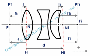Focal lengths are necessary parameters for calculating the paraxial image of a given object.

The front effective focal length f is the algebric distance NF from the front nodal point ( or primary principal point ) N to the front focal point F or from the primary principal plane H to the front focal plane P_f.
The back effective focal length f_i is the algebric distance N_iF_i from the back nodal point ( or secondary principal point ) N_i to the back focal point F_i or from the secondary principal plane H_i to the back focal plane P_fi.

The optical system is said positive (or converging) in the case where the effective back focal length is positive with respect to the direction of the emerging rays. It its said negative (or diverging) otherwise. Sometimes (particulary in ophtalmic optic), focal lengths are replaced by their inverse value which is commonly called the power.

As principal planes are generally not coinciding with a surface of the system, it is also useful to calculate the front and back focal lengths f_t and f_b.

f_t is the algebric distance from the vertex of the first optical surface to the front focal point F.
f_b is the algebric distance from the vertex of the last optical surface to the back focal point F_i.

The front and back focal lengths (not to be confused with front and back effective focal lengths) are not used for optical calculations but for positionning the focal planes regarding a mechanical reference.

Note that the definitions of the front and back focal lengths given above are not standard. For instance, some manufacturers selling mounted lenses may define the front and back focal lengths referred to the mount.

Some other characteristic lengths may be necessary to locate the principal planes referred to mechanical references. They are listed below :

l - distance from the vertex of the first optical surface to the primary principal point N ;
l_i - distance from the vertex of the last optical surface to the secondary principal point N_i ;
d - distance from the primary principal plane H to the secondary principal plane H_i .

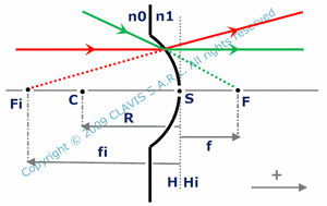A spherical dioptre is a spherical surface interfacting two transparent media. The primary and secondary principal planes coincide with the plane tangent to the dioptre and perpendicular to the optical axis. According to the Snell-Descarte law and applying a first order approximation for small angles, the effective back and front focal length are respectively given by the relations : .
R is the dioptre radius. n₀ and n₁ are the refraction indexes respectively of the object space and of the image space.

Note that according to the definition given in the section "Focal lengths and other parameters", the front and back focal lengths are f_t = f and f_b = f_i.

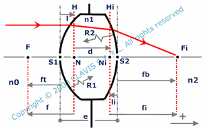Using the Snell-Descarte law with the first order approximation applying in Gauss conditions, the different parameters paraxial parameters are given by the formulas belows. For simplicity, lets define the parameter k :

.

R₁ and R₂ are the respective radii of the first and the second surfaces, n₀ and n₂ are the respective refraction indexes of the object and image spaces, n₁ is the refraction index of the lens and e is the center thickness of the lens.

The positions of the primary and secondary principal planes are given by :

.

The focal lengths are given by the formulas : .

Note that which means that f = - f_i if the object space and the image space have the same refraction indexes and in particular if the lens is used in air or vacuum.

There are lens shapes that give particular results. For example, if the second surface of a lens is plane, the primary principal plane is tangent to the first surface. If the lens is reversed so that the plane surface is the first one, the secondary principal plane is tangent to the second surface.

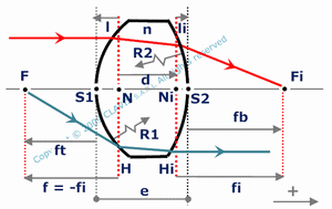The case where the lens is used in the air is the most common case and it is optically very similar to the case where the lens is in vacuum. Then the formulas applicable in the general case are simplified. Indeed, as the refraction indexes of the object and image spaces are equal to 1 :



n is the refraction index of the lens.

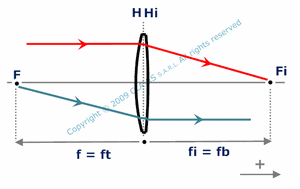A lens is considered as a a thin lens when its center thickness is small enough to be neglected. It is a theoretical case which is however very useful. Here, we consider the case where the lens is in air or vacuum. The vertexes of the lens surfaces coincide. They coincide also with the object and image nodal points. The paraxial parameters are given by the simplified formulas below (the general formula is detailed in the section "Thick lens in the air") :

From the focal length formula, one can see that the lens type (positive or negative) can be easily deducted from its shape. Indeed, for instance, biconvex and plane-convex lenses are positive (f_i positive) while biconcave and plane-concave lenses are negative (f_i negative). A Lens with both convex and concave surfaces is positive if the radius of the convex surface is smaller than the radius of the concave one.

The image of a point at infinity through a positive lens is real, which means that the rays effectively intercept the image focal point while the image through a negative lens is virtual, which means that the rays never "physically" intercept the image focal point but only their directions do.

The effective back focal length of a combination of thin lenses placed one against the other is given by the following formula : where f_ik is the effective back focal length of the lens n°k.

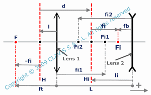
Also, the effective back focal length of a combination of two thin lenses at a distance L from each other is calculated with the formula : (left picture). Therefore, the special configuration where (right picture) gives infinite focal lengths : the system is afocal and the transverse magnification whatever the object is .

In the case of a mirror, principal planes coincide with the plane perpendicular to the optical axis and containing the mirror vertex O. The front and back focal points coincide. Therefore, focal lengths (f, f_i, f_t and f_b ) are then identical : f = f_i = f_t = f_b = R/2 where R is the mirror radius.

The mirror center C is a characteristic point as all light rays coming from C are reflected by the mirror backward in the same direction. The mirror vertex O is also characteristic as it reflects light rays in a symetrical direction regarding the optical axis.

Note that a plane mirror is an afocal system with a magnification of -1.

Basic catadioptric systems are made of a refractive system and a mirror. Light goes first through the refractive system, is then reflected back by the mirror and finally goes through the refractive system a second time in the reverse way.

In its simplest configuration, a catadioptric system is made of a thin lens and a spherical mirror. The whole system is reflective and behaves like a virtual spherical mirror with an equivalent vertex S_eq and an equivalent radius R_eq.

R_eq and the distance x_eq from the lens to S_eq depend on the effective focal length of the lens fi, the mirror radius R and the distance L between the lens and the mirror vertex S_m.

"Optique Fondements et applications" - 2004 - author : José-Philippe Perez.

"Optique géométrique Imagerie et instruments" - 2007 - author : Bernard Balland.

"Optique géométrique paraxiale" - Institut doptique théorique et appliquée - 1985 - author : Michel Cagnet.

"Formation des images Aberrations" - Institut doptique théorique et appliquée - 1985 - author : Michel Cagnet.